Rehashing Kernel Evaluation in High Dimensions
Kernel methods are a class of non-parametric methods used for a wide variety of tasks including density estimation, regression, clustering and distribution testing [1]. In MacroBase, for instance, we use Kernel Density Estimation to perform outlier detection for multimodal data. Despite their wide applications and clean theoretical foundation, kernel methods do not scale well to large scale data: a larger training set improves the accuracy but incurs a quadratic increase in overall evaluation time. This is especially problematic in high dimensions, where the geometric data structures used to accelerate kernel evaluation suffer from the curse of dimensionality.
In this blog post, we summarize results from our recent ICML paper that introduces the first practical and provably accurate algorithm for evaluating Gaussian Kernel in high dimensions, and consequently, achieves up to 11x improvement in query time compared to the second best methods on real-world datasets. Our code is open source on Github.
Problem
We focus on the problem of fast approximate evaluation of the Kernel Density Estimate. Given a dataset \(P=\{x_{1},\ldots,x_{n}\}\subset \mathbb{R}^{d}\), a kernel function \(k:\mathbb{R}^{d}\times \mathbb{R}^{d}\to [0,1]\), and a vector of (non-negative) weights \(u\in\mathbb{R}^{n}\), the weighted Kernel Density Estimate (KDE) at \(q\in \mathbb{R}^{d}\) is given by:
\[\mathrm{KDE}_{P}^{u}(q) := \sum_{i=1}^{n}u_{i}k(q,x_{i}).\]Our goal is to, after some preprocessing, efficiently estimate the KDE at a query point with \((1\pm\epsilon)\) multiplicative accuracy under a small failure probability \(\delta\).
Prior Work
This problem has a long history of study, and we summarize the major lines of related work below:
-
Space-partitioning methods[1][2][3]: This line of work uses geometric data structures to partition the space, and achieves acceleration by bounding the contribution of data points to kernel density using partitions. However, this only works well when the data is in low dimensions, or exhibits intrinsic low dimensionality.
- Random Sampling (RS): In high dimensions, we can get an approximation of the kernel density by taking random samples. In the worst case, an \((1\pm\epsilon)\) approximation of a kernel density of \(\mu\) requires \(O(1/\epsilon^2\mu)\) time.
- Hashing-Based Estimators (HBE): A recent theory paper proposed a new estimator that can achieve the approximation in \(O(1/\epsilon^2\sqrt{\mu})\) time. This result gives the first provable worst-case improvement on random sampling in high dimensions.
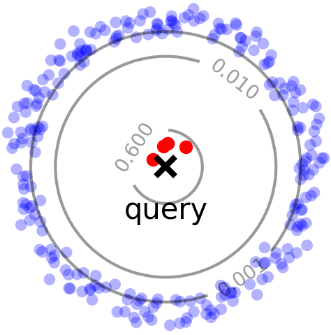
Right: Difficult case for random sampling, where a few close points (red) contribute significantly to the overall density.
A few words on HBE
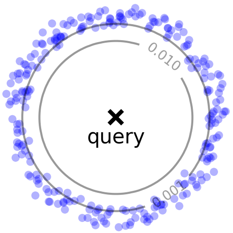
HBE improves upon RS by being able to better sample points with larger weights (kernel values). In particular, RS does not perform well (Figure 1, right) when a significant portion of the density comes from a few points with large weights (close to the query). HBE, instead, samples points proportional to their contribution to kernel density (a.k.a. importance sampling), and therefore has a higher chance of seeing these high-weight points. For radially decreasing kernels, this sampling distribution can be produced via Locality Sensitive Hashing (LSH).
Does theory work in practice?
Given the promise in theory land, we ask, if we implement HBE by the book, does its theoretical gains actually translate into practice? The answer is yes, but with some modifications.
In particular, we found three practical limitations of the HBE: super-linear space usage, large constant overhead of the sampling algorithm, and the use of an expensive hash function for Gaussian Kernels. Below, we outline the challenge and solution to first limitation on space usage, and defer the details of the latter two limitations to the paper.
The preprocessing step of the HBE requires hashing the entire dataset once for each sample it takes, which is prohibitively expensive for large datasets. Instead, we would like to simulate HBE on the full dataset by running it on a representative sample (sketch), which reduces the space usage from super-linear to sub-linear, while still preserving the theoretical guarantees.
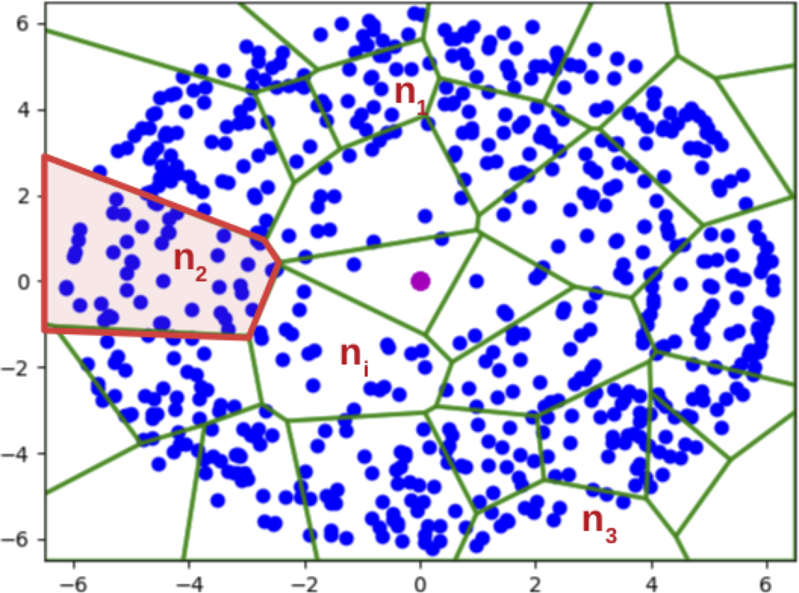
We propose to construct the sketch via hashing (again!) and non-uniform sampling. We illustrate the main ideas of the sketch using Figure 2 (left), which shows a random partition (green polygons) of the dataset (blue dots) under a hash function; each partition is essentially a hash bucket in the hash table.
- If we construct the sketch by simply taking uniform samples from the dataset, we might not have a sample from the sparse regions of the dataset (i.e. some hash buckets have 0 points in the sketch).
- If we construct the sketch by uniformly sampling the hash buckets, we have the opposite problem of overrepresenting small buckets in the sketch, and might need a large number of samples as a result.
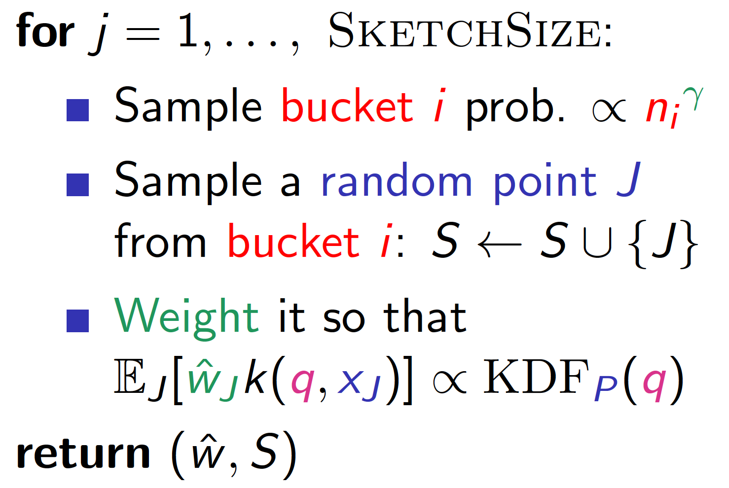
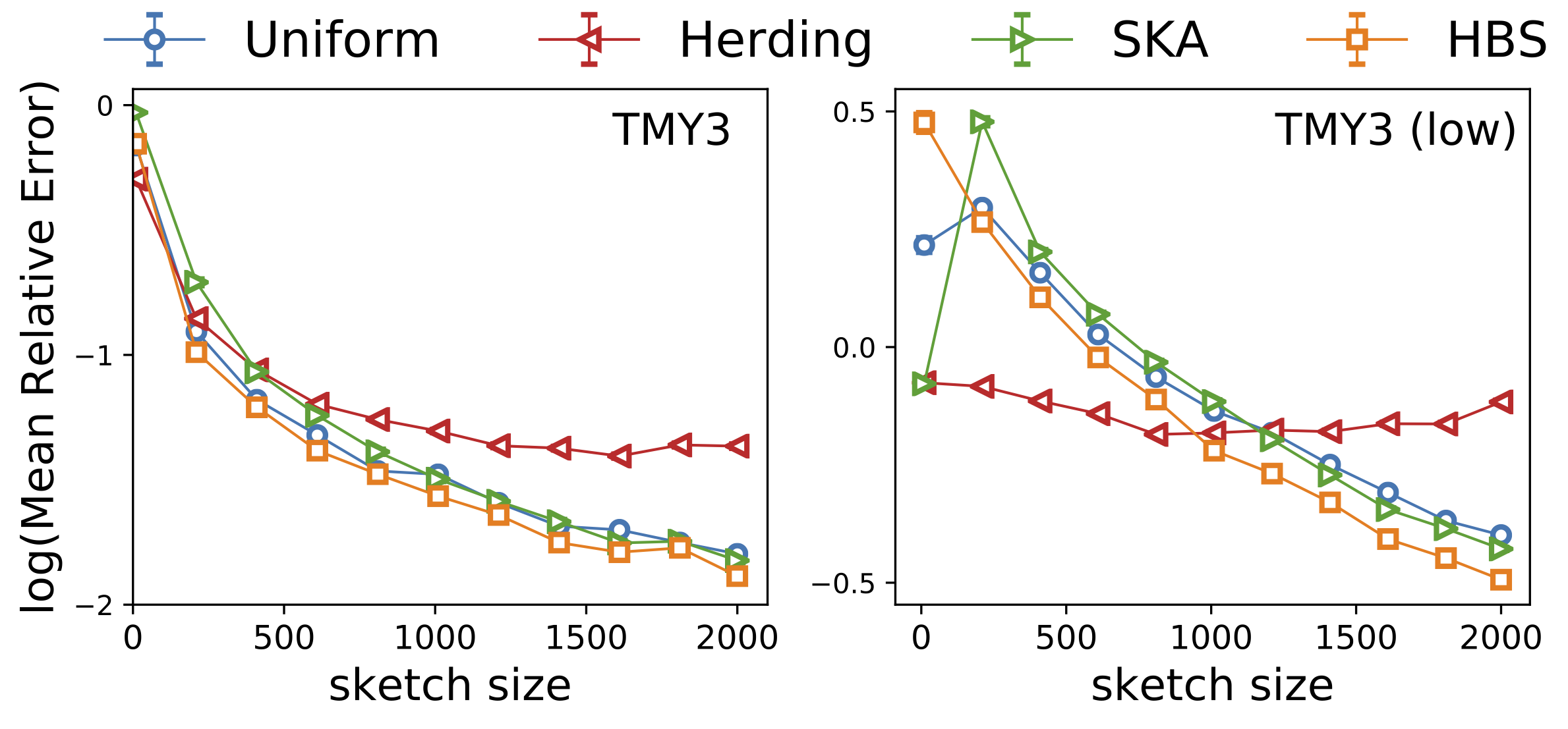
Our Hashing-Based Sketch achieves the best of both worlds through an interpolation of the above two approaches: uniform on the dataset is achieved by setting \(\gamma=1\), while uniform on the buckets is achieved by setting \(\gamma =0\) in the pseudocode (Figure 2, right). We formally proved that with a proper choice of \(\gamma \in (0, 1)\), we are able to sample from any hash bucket that contributes non-trivially to the density, which helps better estimate low-density queries, consistent with our experiment below.
Is it always better to use HBE?
With HBE made much more practical, we further ask: is it always better to use HBE? The answer is no, but there is a way to tell.
The fact that HBE is asymptotically better than random sampling in the worst-case does not mean that it is better for all datasets. For example, for nicely-behaved datasets (Figure 1, left), random sampling might only require \(O(1)\) number of samples to achieve a good estimate of the density, in comparison to \(O(1/\mu)\) in the worst case.
Therefore, the worst-case bounds are insufficient to predict performance on a dataset. In order to determine whether HBE is able to achieve gains on a particular dataset, we need a means to estimate the “hardness” of the dataset. In the paper, we argue that average relative variance is a good indication of the sample complexity of the dataset, and develop a light-weight approach to estimate this metric. The procedure does the following:
- Sample a number of queries from the dataset
- Upper bound the relative variance for each query
- Average the upper bounded relative variance for all queries as a proxy of the sample efficiency
This diagnostic procedure essentially allows us to compare the efficiency of a class of “regular” estimators (which include HBE and RS) on a given dataset. Interestingly, the new variance bound we developed in step 2 of the procedure also allows us to simplify and recover the results of the original HBE paper!
Results
We evaluate on a number of real-world and synthetic datasets. With HBS, the preprocessing time of HBE becomes on part with alternative methods. We focus on comparing query time to achieve the same accuracy in the evaluations below.
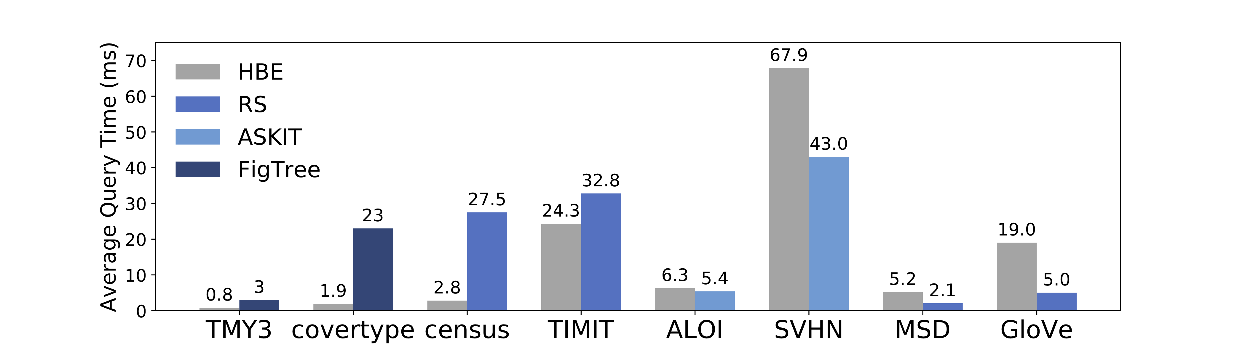
On a set of real-world datasets with varying size and dimensions (Figure 4), HBE is always competitive with alternative methods and is faster by up to 11x over the second best method.
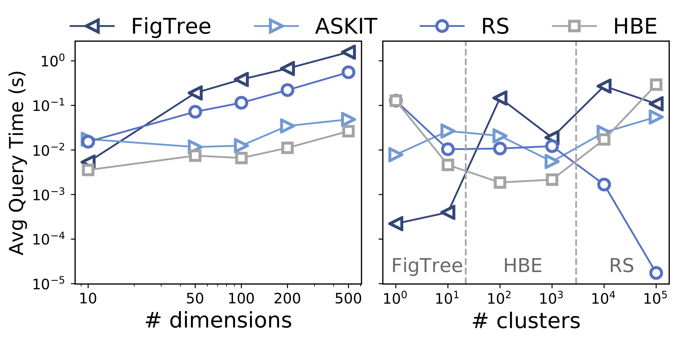
On a set of “worst-case” synthetic benchmarks (Figure 5, left), HBE consistently outperforms alternatives. On a set of synthetic benchmarks with varying number of clusters (Figure 5, right), HBE performs the best on datasets with “intermediate” cluster structures, while RS and space-partitioning methods excel at the two extremes of highly clustered and highly scattered datasets.
In addition, we have tested the diagnostic procedure on a total of 22 real-world datasets, among which the procedure correctly predicts the more sample efficient estimator for all except one dataset.
Summary
In this post, we give a glimpse of the work that went into making a theory paper practical, as well as the new theoretical results inspired by practical constraints. Overall, our modified HBE achieves competitive and often better performances at estimating kernel densities on real and synthetic datasets. Please check out our paper and the supplementary materials for additional details and experiments. Our code is also available as open source on Github.