Sketching Classifiers with Limited Memory, or Better Feature Hashing with One Simple Trick

This post accompanies the paper “Sketching Linear Classifiers over Data Streams” by Kai Sheng Tai, Vatsal Sharan, Peter Bailis and Gregory Valiant, which was presented at SIGMOD 2018. Check out our code on GitHub.

In online learning, we learn a predictor by continuously updating its weights according to a stream of labelled examples. For example, in spam classification, an online learning approach allows the spam classifier to dynamically adapt to newly-observed features, even those introduced by an adversary attempting to evade detection. In memory-constrained environments such as mobile or embedded devices, there exists an important trade-off between classification accuracy and the memory footprint of the classifier. In this post, we describe a simple technique that improves on a standard method for learning memory-budgeted classifiers called feature hashing. The idea is to introduce a coarse-to-fine approximation by augmenting the hashed weight vector with a heap that stores important, high-magnitude model weights. Controlling for the available memory budget, we show that this simple extension achieves consistent accuracy improvements over feature hashing on several real-world datasets.

Linear classification with limited memory

Linear classifiers are an essential part of the modern machine learning toolbox. Given a good set of input features, linear models such as logistic regression, naïve bayes and linear SVMs have been used to achieve excellent classification accuracy on important prediction tasks like spam detection, ad click-through-rate prediction, and network traffic classification. As an added bonus, we can often interpret the weights learned by these linear models as indications of relative feature importance, a useful metric for meta-tasks like debugging poor model performance.

Memory usage isn’t typically considered a bottleneck when we’re deploying linear classifiers in server environments. However, memory constraints can quickly become a key limitation on mobile and embedded platforms. As an extreme example, the popular Arduino Uno microcontroller board ships with a measly 2KB of onboard RAM. Other devices like the Google Home or the Amazon Echo impose less stringent memory limits, but are still at least an order of magnitude more memory constrained than typical commodity server hardware. Despite these hardware limitations, there is growing interest in on-device learning and inference—for example, a recent paper from Microsoft describes how tree models can be tailored for deployment on the Uno. On-device learning offers interesting new possibilities for ML-based systems—for instance, predictive systems that can adapt to local observations without needing an internet connection, or on-device models that can be quickly personalized to the peculiarities of individual users.

If we were only interested in performing inference on a memory-constrained platform using a classifier that is trained “offline,” then well studied feature selection techniques can be used to optimize for the classification accuracy of the classifier under the given memory budget. The problem is more challenging in the online learning regime, where we want classifiers that adapt on-the-fly to a stream of new examples. This is particularly relevant to applications where we expect that the distribution of features and labels will change over time. For example, in a network traffic classification task, we may expect that the distribution of features derived from headers and other packet-level data will change due to variations in user behavior, or due to intentional manipulation by malicious users—in order to retain high classification accuracy, a classifier should be continuously tuned according to newly-observed data.

Hash all the things

There’s a simple but effective trick that guarantees a classifier will never exceed a given memory constraint—even in the challenging online setting—while providing decent classification performance in practice. This trick goes by several names: feature hashing, hash kernels, and the hashing trick. The main idea is the following. Choose a hash function \(h(i)\) that maps from keys \(i\) to the integers \(\{1, 2, \dots, k\}\), and a second, independent hash function \(s(i)\) that maps from keys to \(\{-1, +1\}\). Given a feature vector \(x\), define the hashed feature vector \(\tilde{x}\) as:

In words, hash each index \(i\) to a bin \(h(i)\) and add the value \(x_i\) multiplied by a random sign flip. Instead of learning a classifier over the original high-dimensional feature space, we’ll instead learn a classifier over the hashed, \(k\)-dimensional feature space. Since a linear classifier over \(k\)-dimensional feature vectors can always be represented using \(O(k)\) bits, by choosing a small enough \(k\), we guarantee that the classifier will never exceed the prescribed memory limit. For example, in a text classification task, the raw feature vectors might be indexed by n-grams like “quick brown fox” and “the lazy dog”. We could hash these strings to 16-bit values and learn a classifier over a feature space of dimension \(2^{16}\). In this case, about 262KB of memory is needed to represent the classifier weights using 32-bit floats.

As with all hashing-based techniques, collisions are the bane of feature hashing. Since a single weight is learned for all features that hash to the same bucket, the classification error increases as the number of buckets \(k\) decreases. Another drawback is the loss of model interpretability—since multiple features hash to the same bucket, they cannot be differentiated for the purposes of inferring feature importance from the model weights. If we think of the classifier trained on the hashed features as being a compressed version of the hypothetical classifier trained on the original, high-dimensional features, then this problem can be seen as the inability to uncompress or recover the original classifier from its compressed form.

Collision avoidance with one simple trick

Notice that in our formulation of feature hashing, we only used a single pair of hash functions, \(h(i)\) and \(s(i)\). In our SIGMOD paper, we analyze a variant of feature hashing that instead uses multiple hash functions—by hashing using sufficiently many independent hash functions, it turns out that we can in fact approximately recover the original classifier from the compressed version learned on the hashed feature space. We draw a connection between this method and to a long line of previous work in sketching algorithms for streaming data, hence the name for our multiple-hashing method for learning compressed linear classifiers: the Weight-Median Sketch, or WM-Sketch for short.

In this post, we will highlight a surprising empirical finding from our work (for readers more interested in the theoretical aspects of our analysis, more details are available in the paper). Here’s the punchline:

To improve on standard feature hashing, use a heap to track the highest-magnitude weights in the model.

For the sake of brevity, we’ll call this technique the “heap trick.” Given a memory budget of \(K\) bytes, standard feature hashing uses the entirety of the budget to store the array of weights corresponding to the hashed features. Instead, we will reserve \(K/2\) bytes for a min-heap of (key, weight) pairs \(\left(i, w_i\right)\) ordered by the weight magnitudes \(\lvert w_i \rvert\). Note that the keys here are from the original, high-dimensional feature space; for concreteness, we assume that each \(i\) is represented by a 32-bit integer. The remaining \(K/2\) bytes are used for an array of weights as in standard feature hashing.

The update scheme is simple. During stochastic gradient descent (SGD) or online gradient descent (OGD), we adjust the model weights to minimize a given loss function. If the weight to be updated is present in the heap, the corresponding value is updated exactly. Otherwise, the key is hashed and the resulting bucket in the array is updated. If, after the update, the weight is larger in magnitude than the smallest-magnitude weight currently stored in the heap, the smallest-magnitude weight in the heap is replaced with the weight estimated from the hash-array.

The intuition behind this technique is that high-magnitude weights have the largest influence on the classification decision. When an important, high-weight feature collides with an unimportant, low-weight feature, we suffer from increased classification error. In contrast, we therefore, by storing them in the heap where there is no possibility of hash collisions, we can reduce the error incurred by the compressed representation of the classifier. In other words, the heap attempts to capture the largest-magnitude weights, while the hash-array approximates the tail of the weight distribution.

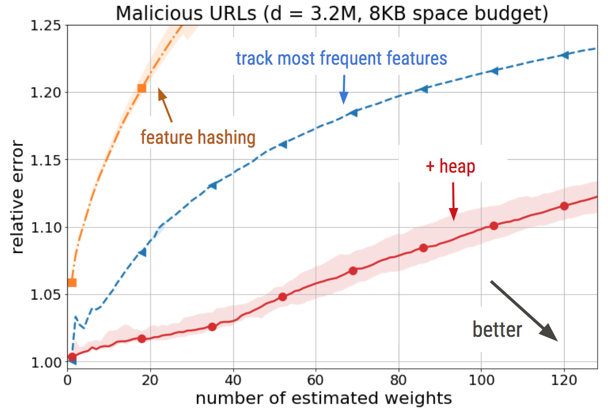
How does this simple trick perform empirically? We trained an L2-regularized logistic regression classifier on a malicious URL detection dataset (with original feature dimensionality of 3.2 million) using online gradient descent and measured the online error rate of each classifier.

We find that the addition of the heap improves on feature hashing by a small but consistent margin across all the memory budgets we tested.

We can also test how well the recovered model weights approximate the weights of the classifier trained without any memory constraints. Here, we find that the weights that percolate up into the heap are in fact a good approximation of the highest-magnitude weights in the uncompressed classifier.

In our SIGMOD paper, we report further experimental results on a text classification dataset and on a KDD large-scale data-mining dataset with over 20 million features. In all cases, we observed a consistent improvement over feature hashing in terms of classification accuracy, while providing improved model interpretability by approximating the highest-magnitude weights that would have been learned had we trained the classifier without any dimensionality reduction via hashing.

Takeaways

In this post, we described how an extremely simple trick can realize surprising improvements in both accuracy and interpretability over standard feature hashing, a commonly-used technique for reducing the memory usage of linear classifiers.

In the paper, we also describe how this method can be applied to several streaming, memory-limited analytics tasks. In particular, we show how tasks like detecting highly-correlated events can be formulated as classification problems on data streams, and are therefore amenable to techniques such as the heap trick explained here.

Our hope is that techniques for learning more accurate memory-boxed classifiers, such as those described here and in the paper, will encourage practitioners to think of more resource-constrained applications that could nevertheless benefit from a light dusting of ML.