Debugging Training Data for Software 2.0
Training data is playing an increasingly important role in defining the performance of modern machine learning systems. The goal of this blog post is to maintain a “checklist” of the types of errors that can be introduced by unaccounted phenomena in the data and their labels, and simple ways to check for these errors. We would love to hear about other errors you have encountered and how you identify and correct them!
Check out our previous blog on using the lineage of training data to detect errors!
This blog is a work in progress and a list of the different errors and potential solutions we have heard about from collaborators. We want to keep adding to this based on your feedback and experiences!
In traditional software engineering, or Software 1.0, a program’s functionality is defined via code as dictated by a human. In the age of machine learning, we are increasingly observing Software 2.0 systems, where a program’s functionality is defined by the weights of neural networks as dictated by the data[1], [2], [3]. You wouldn’t trust a piece of human-written code that hasn’t ever been debugged or tested, so why shouldn’t our data receive the same treatment now that it’s a first-class citizen in so many real-world systems?
To that end, this blog post is about “debugging” data — systematically identifying and removing sources of error in machine learning models caused by phenomena in the data and/or their labels. Our checklist is inspired by our readings[1], [2], [3], recent blogs, and our own experiences with managing and shaping training data[1], [2], [3], [4]. We’d love to add to it as you share with us other data bugs you’ve observed!
Updates 09/27/18
-
Google’s new What-If Tool offers an interactive visual interface for users to explore and debug their data and machine learning model. We view it as a “dashboard for machine learning”, allowing users to understand their data and model without writing a lot of code.
-
We chatted with industry affiliates of DAWN at the recent retreat and heard their thoughts about debugging in machine learning - a summary of our conversations here!
Types of Data and Label Errors
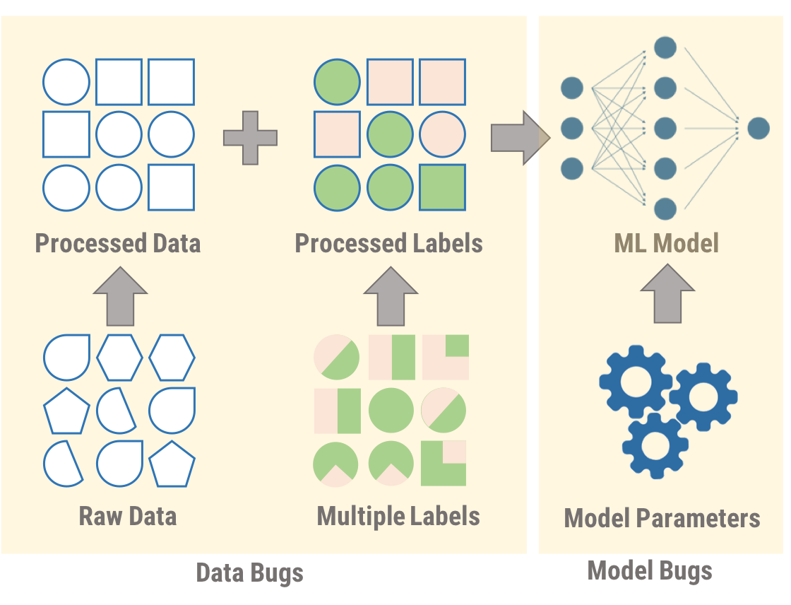
We begin by separating data bugs into three categories, and defining different problems that fall into these categories:
- Data Errors
- Data Split Errors (given single label per datapoint)
- Label Errors (given multiple labels per datapoint)
It is also possible to have bugs in a machine learning model itself; however, in this blog, we focus only on errors in the data and their corresponding labels. This checklist is not meant to be complete, but a starting point to gather information about data errors and solutions from ML practitioners.
P.S. The blog post is a bit lengthy, the links above should help navigate!
Data Errors
The first class of errors is data errors; even before we have labels, it’s possible (and often likely) that our dataset contains certain examples which will hurt performance no matter how they’re labeled. We cover the following error types and potential solutions:
Problem: Unwanted Outliers in the Data
The dataset can have unwanted outliers that can degrade the performance of the classifier. Suppose I’m training a dog breed classifier and my dataset includes the following image as as one out of five examples for a particular breed. Do I want to train my classifier to learn to associate the features related to a dark background with a particular breed? The answer depends on the kind of data we will eventually use our model for and what kind of examples we want it to be robust to.

Solution
To find anomalies such as these, the most straightforward approach is to simply plot all your data points on as many axes as you can think of—for example, by average pixel intensity or file size, or by word length or number of capitalized words. Or use a dimensionality reduction technique like t-SNE and view the resulting embeddings. With each of these plots you’re just looking for anomalies–unexpected spikes, loners, and strange clusters.
We could also inspect the training loss of the model to see whether the loss seems to plateau after encountering a specific example, and cluster all such examples to find interesting characteristics. Once important axes of variation are identified, several distinct approaches can be used to mitigate the effect of unwanted outliers:
- Removal: Outliers can simply be removed from the dataset if they truly are not representative of the population expected at test time. In the example above, we could simply remove images with poor lighting. Or for a more principled approach, we could apply “data dropout”[1], a two-stage process where training examples that hurt performance on the validation set are identified automatically and removed before repeating training on the pruned training set.
- Augmentation: Data augmentation is a critical component towards achieving state-of-the-art results with many modern machine learning approaches[1], [2]. In the context of debugging, this process entails observing non-uniform variation of the dependent variable (i.e. dog breed) along a particular axis (i.e. lighting) and augmenting the training dataset with transformed or synthetic points such that the dependent variable is no longer correlated with variation along a non-desirable axis. For our dog breed classifier, this could involve finding or creating images of each dog breed at different levels of lighting and adding these to the training dataset.
- Alignment: Alignment represents the opposite approach to augmentation – instead of choosing to fully populate a given axis of variation such that it is no longer correlated with the dependent variable in the training set, we can also choose to perform transformations on the data that eliminate variation along that axis altogether. This is particularly common in image analysis, where images are often normalized before input into a training procedure to eliminate the effects of specific imaging hardware (e.g. camera or scanner type), context (e.g. different color statistics for pathology slides that come from different institutions), or postprocessing (e.g. selective filtering for reconstructed volumetric images). In our dog breed example, this could perhaps involve performing histogram equalization or mean-standard deviation normalization on each image to eliminate the effects of different sensors (cameras), contexts (background lighting), and postprocessing (photo editing) on our learning process.
Problem: Errors in Converting Raw Data to Processed Data
It is common for the raw data to be processed before inputting it into a classifier (or even assigning labels) and errors can occur during this process. Consider classifying sentences in which the format of the source documents results in the same sentence “All Rights Reserved” being produced at the end of each one. I probably don’t want to have N identical copies of this sentence in my training data.
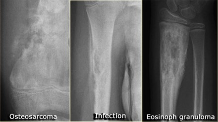
Other problems in the Extract-Transform-Load (ETL) process iinclude incorrect data normalization or not cropping metadata like tags in a medical image, which leads the classifier to rely on the metadata rather than the content of the image for classification. Imagine training a classifier for identifying the grade of bone tumors in X-rays using a dataset where most of the examples of a certain class occur in the arm. If images are not cropped properly, the classifier can learn features for the arm rather than the tumor itself. Further, if the image normalization process happened to cause extremely large or nonsensical pixel values (e.g. NaN, Inf, etc.) in even one example, the resulting gradient explosion during training process can substantially decrease model performance.
Solution
While most problems in the data processing pipeline are domain specific, one generic way to check for errors in this process is to cluster the data and make sure the distribution is the same before and after processing, using tools like t-SNE or measuring statistical differences between distributions. If possible, training a simple classifier on both the raw and processed data and comparing performance is also helpful. For example, processing the data should help classifier accuracy, not hurt it!
Additionally, we have found that in practice, gradient clipping can be a helpful way to ensure that even needle-in-a-haystack ETL errors do not degrade end model performance by causing massive parameter changes due to a spuriously exploding gradient.
Problem: Corrupted Data Fields
With structured data, especially data that has been entered by humans, there are often corrupted entries in the data. Consider, for example, the following table (borrowed from the HoloClean blog):
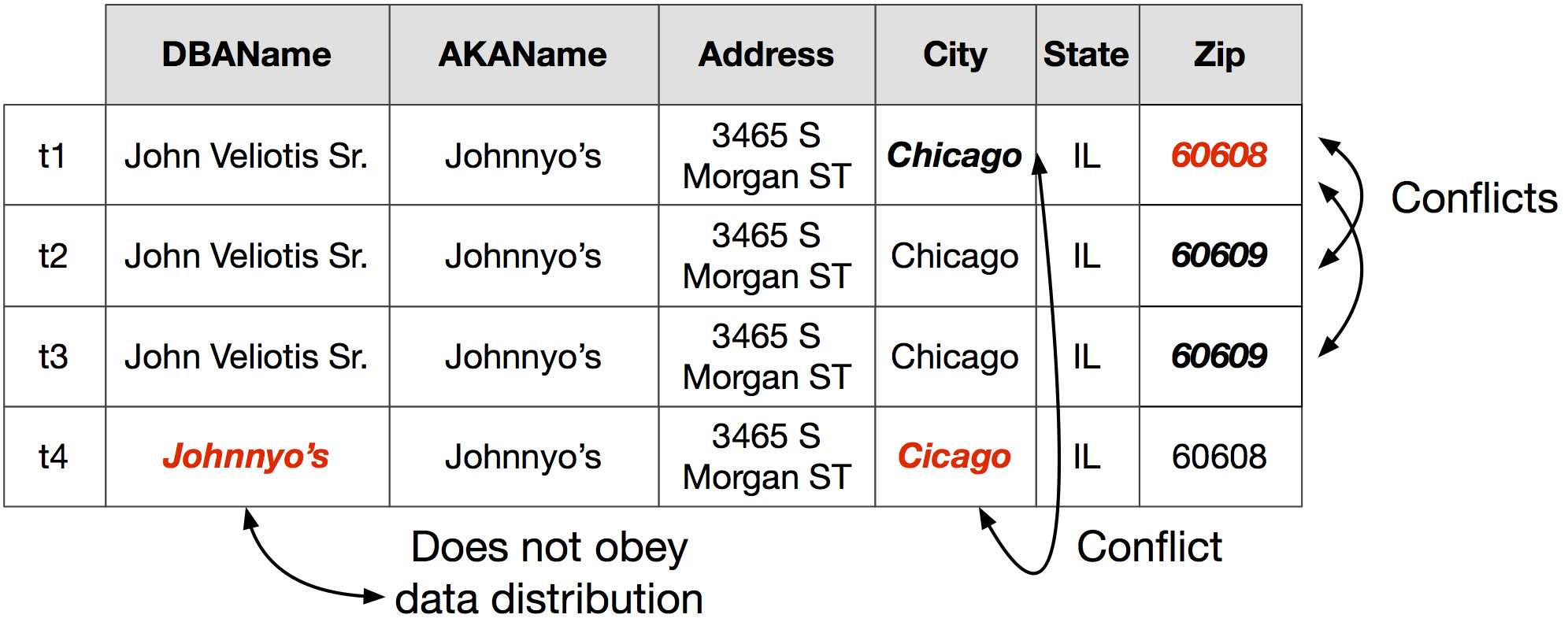
Solution
Situations like these present an opportunity for data cleaning, including automated approaches such as HoloClean, BoostClean, and systems from companies like Tamr and Trifecta.
Problem: Data from Multiple Sources
Often data is collected from multiple sources, which can lead to training a “data source classifier” instead of a true classifier. For example, there’s an old machine learning urban legend about the military trying to train a classifier to recognize allied vs. enemy tanks. The classifier was a huge success–over 95% accuracy! They deployed it, then soon found that it performed no better than random chance. How is that possible? The allied tanks were photographed on Monday on a sunny day, whereas the enemy tanks were photographed on Tuesday when it was cloudy. Consequently, their classifier had simply become a brightness classifier.
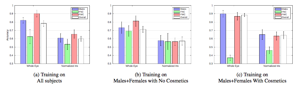
A similar situation is reported in the gender-from-iris paper, where a classifier for identifying gender based on the irises was actually found to rely heavily on the presence of makeup around the eyes. We have observed similar results in practice in problems in medicine, wherein small differences like the color statistics of different batches of a chemical staining agent used in otherwise similar imaging procedures can result in classifiers that miss the clinically important variables while “accurately” predicting the appropriate outcome based on strong associations between color statistics and the institution from which an image is sourced.
Solution
Any time that your data comes from multiple sources (and therefore potentially multiple source distributions), you should be wary of differences that may cause your classifier to become a “source classifier” rather than a classifier for the effect you actually care about.
Normalizing or whitening your data (where applicable) can remove some of the obvious clues about sources, but these processes usually won’t remove all such clues. Segmenting only the area of interest for classification is another possible solution, but may result in other unwanted issues. In case of classifying data from people, creating person-disjoint train and test sets can prevent the model from overfitting to patient-specific characteristics as well (sometimes this is okay, more in this section). Another simple sanity check is to create a classifier to explicitly predict the data source from the data at hand – if this can be easily accomplished, it may be a clue that this problem is affecting your results.
Data Split Errors (given single label per datapoint)
The second class of errors is errors in the the way the data is split among train, validation, and test and how the different classes are defined and labeled. In this case, we assume that we only have access to a single label per datapoint and have a model trained on this data. We can use the distribution of the data as well as results of the trained model to identify such errors. Even if your labels individually are correct, there are a number of ways that you can shoot yourself in the foot if you’re not careful about the way you create your splits of data for training, validation, and testing:
Problem: Biased Training, Validation, and Test Set Split
Even when the data is clean, the way the data is split across the train, validation, and test set when training a model can lead to over or underestimating the true performance of the model in the real world.
Training vs. Validation: Consider predicting the selling cost of houses based on a number of properties, and the dataset is sorted by zip code. If one makes an 80/10/10 split of the data without shuffling first, they will have no West Coast zip codes in the training set and all of them in the validation/testing sets. Given that houses on the coasts are generally more expensive than properties in the interior, this will likely throw off the algorithm.
Solution
Randomly shuffle the data to create the training and validation sets to ensure the each data split is a representation of the underlying distribution. In some cases when retraining is not too expensive, cross validation can also help.
Validation vs. Test: For the validation set to serve its purpose, it needs to be as close a proxy to the test set as possible. Imagine I’m trying to improve the search engine on my website and I have a small amount of true labels from real user interactions (when users rated the relevance of the returned results). Not wanting to make my test set any smaller, instead of splitting it I label an additional validation set on my own. But unsurprisingly, I’m a little kinder in my evaluation of my own system than my users are, and consequently the validation set has 80% of results marked as acceptable whereas the test set only has 70%. When I tune my model based on the validation set, my model will learn to reflect the prior that about 80% of inputs will be classified as acceptable, and this will cause cause performance to suffer on the test set where that is not the case.
Problem: Dependent Data across Different Splits
Despite randomly splitting data, there can be hidden dependencies between the training and validation set that affect model performance. From the previous two bullets in this section, it may seem like the best approach is to make my data splits by performing random sampling from a single homogenous pool of data; unfortunately, even this approach has its pitfalls!
A common example of dealing with dependent data occurs when we have multiple data points for a single user or patient. Specifically, if we randomly allocate data points to our different splits, we will likely end up with points from the same individual in each set. The model will achieve a high score on the validation and test sets by essentially “memorizing” a particular patient’s data, which is not representative of its performance in the real world.
In some contexts (i.e. if we want a model that predicts on patient X given previous history of patient X), having data from the same patient across splits is fine; in others (we want to predict on patient Y given data on patients A, B, C, etc.), it will cause us to substantially overestimate model performance.
Solution
Various good practices such as regularization on features, data anonymization, or removing too infrequent features can mitigate it, but there are many other scenarios where this source of error can manifest itself. And the way to correct it is to acknowledge the fact that in some scenarios, not all data points are independent–they may be sentences from the same document (with a shared topic) or articles from the same author (with a shared vocabulary). We would like our validation and test set to be as similar as possible, but when it comes to creating our training set, it’s generally good practice to make sure that dependent data points find themselves all the way in or all the way out of the set, so as to avoid this “leaking” of information that promotes memorization over learning. Additionally, strategies such as splitting by user (e.g. ensuring all data from a given user is in the same split) or temporal splitting (attempting to predict at time t+1 based on data from time t) can be useful in creating training datasets that accurately reflect the appropriate problem setup.

Problem: Imbalanced or Conflated Classes
Even if you only have access to a single label per datapoint, there can be issues in the distribution of datapoints among different classes. Suppose I’m building a multi-class classifier to identify different types of dogs. A simple histogram of the different classes in the training data can show me that I only have 1-2 examples of Tibetan Mastiffs. Because of the lack of examples for one class, the classifier performs very poorly at identifying Tibetan Mastiffs, hurting the overall performance of the model.
Another possible issue is when two classes are too difficult to distinguish, as illustrated by the Silky and Yorkshire Terriers in this blog. Although the error is coming mostly from a difficult classification task, this can lower the score of the overall model.
Solution
To correct such problems, we can intentionally collect more instances of that class, subsample the majority class, or oversample the minority class to create a more even class balance. We could also merge classes into broader categories (if applicable). On the model side, we can adjust the loss function of the machine learning model to more highly value getting minority classes correct or change the scoring metric (using F1 or DCG scores instead of accuracy).
Label Errors (given multiple labels per datapoint)
Finally, the third class of errors we explore is when we have access to multiple labels per datapoint. Our previous blog post discusses how we can use provenance of how these labels are generated to debug them. This includes:
Increasingly, labels for training data are gathered via several noisy sources like crowdworkers, heuristics, or simpler models. Our previous work looks are natural language explanations as sources of labels, as well as programmatic functions through Snorkel.
We thank Erik Meijer, Daniel Kang, Fred Sala, Ann He, Vincent Chen, and many members of Hazy Research for their insightful discussions and feedback!