Hyperbolic Embeddings with a Hopefully Right Amount of Hyperbole
Check out our paper on arXiv, and our code on GitHub!
Valuable knowledge is encoded in structured data such as carefully curated databases, graphs of disease interactions, and even low-level information like hierarchies of synonyms. Embedding these structured, discrete objects in a way that can be used with modern machine learning methods, including deep learning, is challenging. Fundamentally, the problem is that these objects are discrete and structured, while much of machine learning works on continuous and unstructured data.
Recent work proposes using a fancy sounding technique—hyperbolic geometry—to encode these structures. This post describes the magic of hyperbolic embeddings, and some of our recent progress solving the underlying optimization problems. We cover a lot of the basics, and, for experts, we show
- a simple linear-time approach that offers excellent quality (0.989 in the MAP graph reconstruction metric on WordNet synonyms—better than previous published approaches—with just two dimensions!),
- how to solve the optimal recovery problem and dimensionality reduction (called principal geodesic analysis),
- tradeoffs and theoretical properties for these strategies; these give us a new simple and scalable PyTorch-based implementation that we hope people can extend!
Hyperbolic embeddings have captured the attention of the machine learning community through two exciting recent proposals. The motivation is to combine structural information with continuous representations suitable for machine learning methods. One example is embedding taxonomies (such as Wikipedia categories, lexical databases like WordNet, and phylogenetic relations).
The big goal when embedding a space into another is to preserve distances and more complex relationships. It turns out that hyperbolic space can better embed graphs (particularly hierarchical graphs like trees) than is possible in Euclidean space. Even better—angles in the hyperbolic world are the same as in Euclidean space, suggesting that hyperbolic embeddings are useful for downstream applications (and not just a quirky theoretical idea).
In this post, we describe the exciting properties of hyperbolic space and introduce a combinatorial construction (building on an elegant algorithm by Sarkar) for embedding tree-like graphs. In our work, we extend this construction with tools from coding theory. We also solve what is called the exact recovery problem (given only distance information, recover the underlying hyperbolic points). These ideas reveal trade-offs involving precision, dimensionality, and fidelity that affect all hyperbolic embeddings. We built a scalable PyTorch implementation using the insights we gained from our exploration. We also investigated the advantages of embedding structured data in hyperbolic space for certain tasks within natural language processing and relationship prediction using knowledge bases. We hope our effort inspires further development of techniques for constructing hyperbolic embeddings and incorporating them into more applications.
What’s Great About Hyperbolic Space?
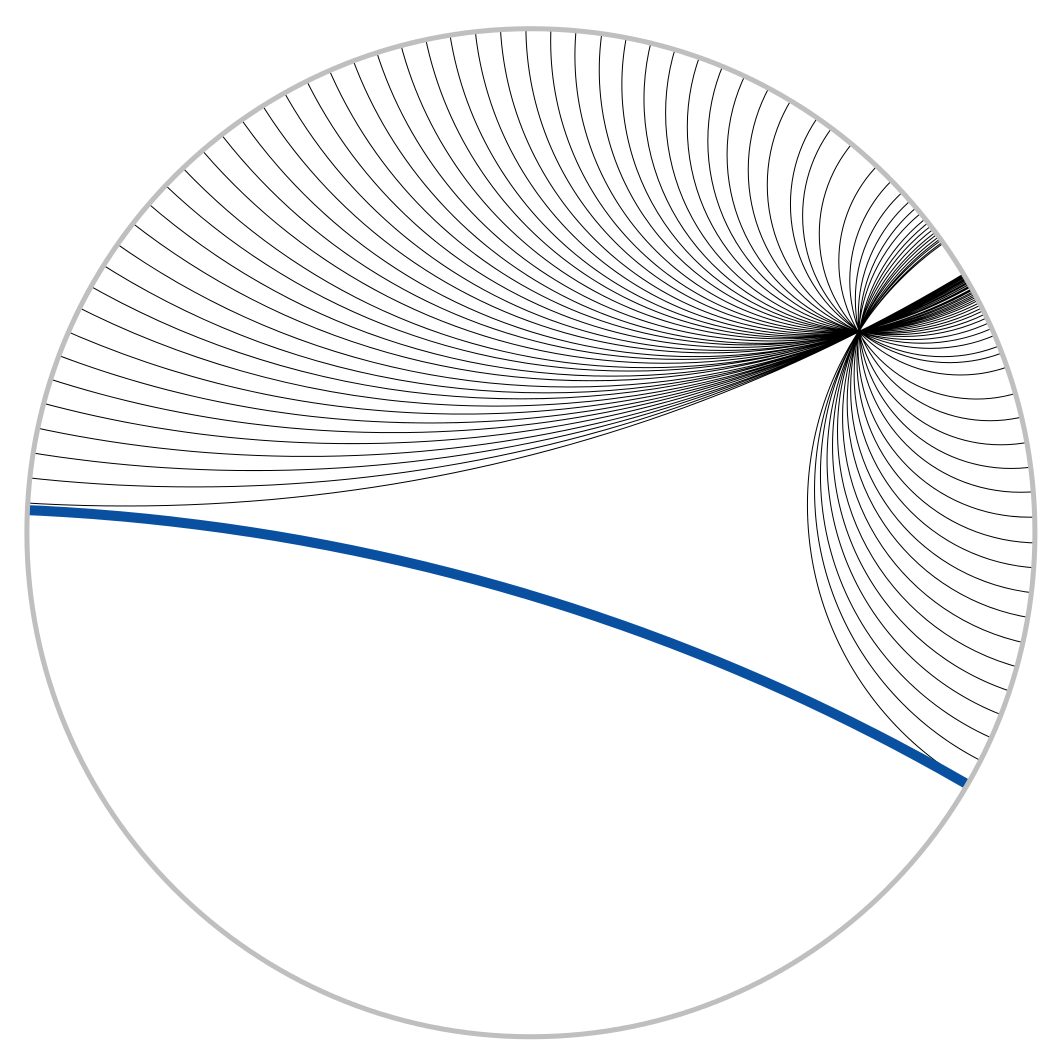
Following prior work, our hyperbolic spaces of choice are the Poincaré disk, in which all points are in the interior of the unit disk in two dimensions, and the Poincaré ball, its higher-dimensional cousin. Hyperbolic space is a beautiful and sometimes weird place. The “shortest paths”, called geodesics, are curved in hyperbolic space. The figure shows parallel lines (geodesics); for example, there are infinitely many lines through a point parallel to a given line. The picture is from the Wikipedia article that contains much more information (or see Geometry).
The hyperbolic distance between two points \(x\) and \(y\) has a particularly nice form: \[ d_H(x,y) = \mathsf{acosh}\left(1+2\frac{\|x-y\|^2}{(1-\|x\|^2)(1-\|y\|^2)} \right). \]
Consider the distance from the origin \(d_H(O,x)\). Notice as \(x\) approaches the edge of the disk, the distance grows toward infinity, and the space is increasingly densely packed. Let’s dig one level deeper to see how we can embed short paths that define graph-like structures—in a much better way than we could in Euclidean space.
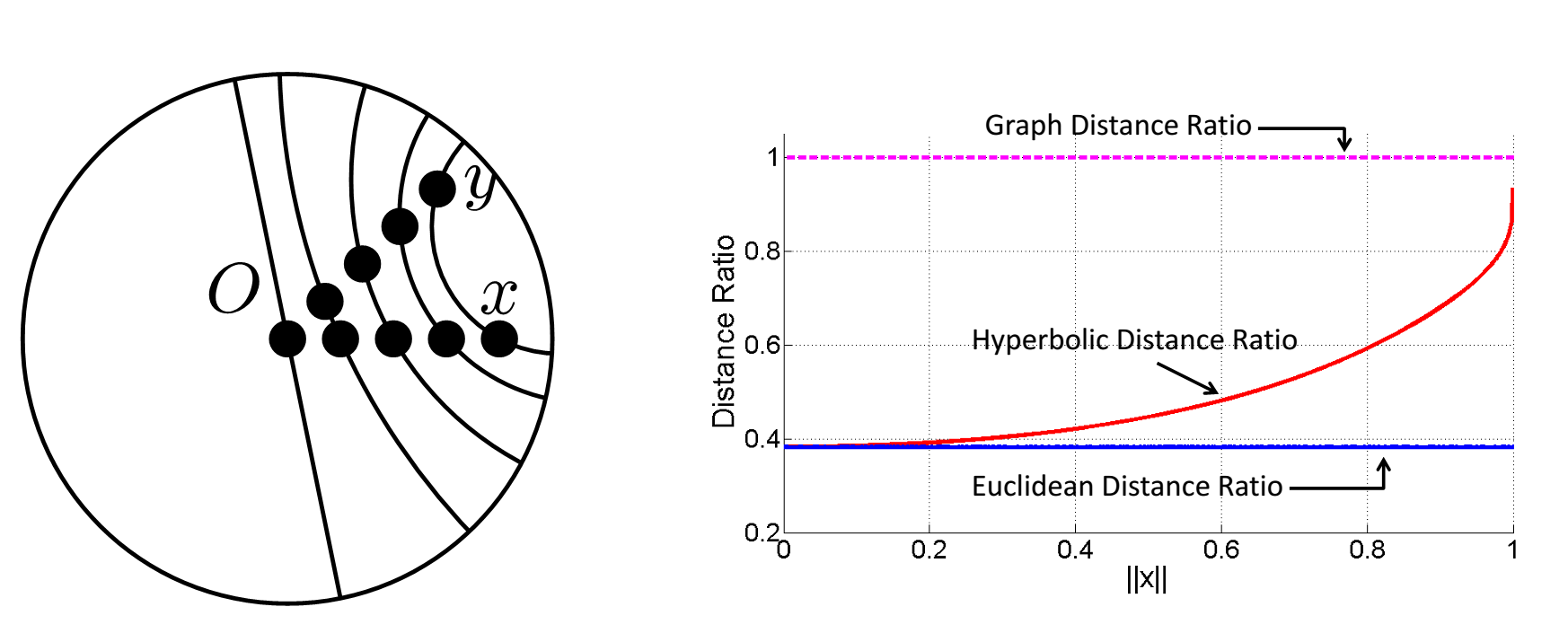
The goal when embedding a graph G into a space \(V\) is to preserve the graph distance (the shortest path between a pair of vertices) in the space \(V\). If \(x\) and \(y\) are two vertices and their graph distance is \(d(x,y)\), we would like the embedding to have \(d_V(x,y)\) close to \(d(x,y)\). Now consider two children \(x\), \(y\) of parent \(z\) in a tree. We place \(z\) at the origin \(O\). The graph distance is \(d(x,y) = d(x,O) + d(O,y)\), so normalizing we get \(\frac{d(x,y)}{d(x,O)+d(O,y)} = 1\). Time to embed \(x\) and \(y\) in two-dimensional space. We start with \(x\) and \(y\) at the origin, and with equal speed move them toward the edge of the unit disk. What happens to their normalized distance?
In Euclidean space, \(\frac{d_E(x,y)}{d_E(x,O)+d_E(O,y)}\) is a constant, as shown by the blue line in the plot above, so Euclidean distance does not seem to capture the graph-like structure! But in hyperbolic space, \(\frac{d_H(x,y)}{d_H(x,O)+d_H(O,y)}\)(red line) approaches \(1\). We can’t exactly achieve the graph distance in hyperbolic space, but we can get arbitrarily close! The trade off is that we have to make the edges increasingly long, which pushes the points out the edge of the disk. Now that we understand this basic idea, let’s actually see a simple way to embed a tree due to a remarkably simple construction of Sarkar.
A Simple Combinatorial Way to Create Hyperbolic Embeddings. Sarkar knows!
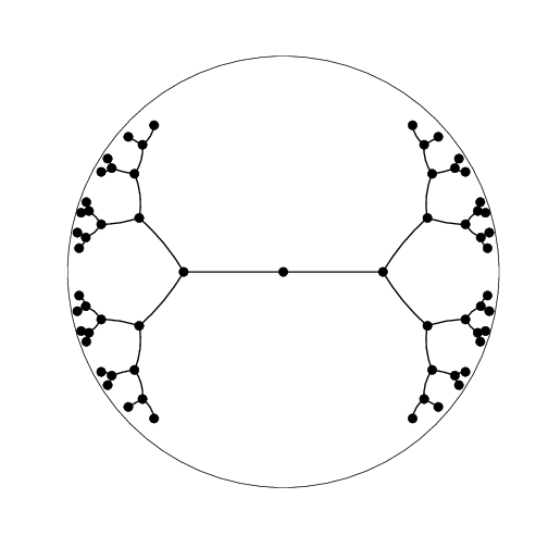
Since hyperbolic space is tree-like, it’s natural to consider embedding trees—which we can do with arbitrarily low distortion, for any number of dimensions! In our paper, we show how to extend this technique to arbitrary graphs, a problem with a lot of history in Euclidean space. We use a two-step strategy for embedding graphs into hyperbolic space:
- Embed a graph G = (V, E) into a tree T.
- Embed T into the Poincaré ball.
To do task 2, we build on an elegant construction by Sarkar for two-dimensional hyperbolic space; we call this the combinatorial construction. The idea is to embed the root at the origin and recursively embed the children of each node in the tree by spacing them around a sphere centered at the parent. As we will see, the radius of the sphere can be set to precisely control the distortion.
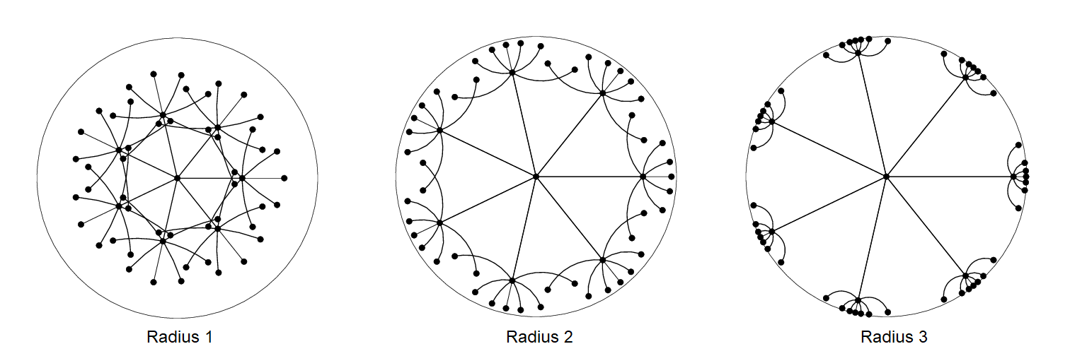
There are two factors to good embeddings: local and global. Locally, the children of each node should be spread out on the sphere around the parent. Globally, subtrees should be separated from each other; in hyperbolic space, the separation is determined by the sphere radius. Observe as we increase the radius (from 1 to 2 to 3), each subtree becomes increasingly separated:
How do we precisely measure the quality of an embedding? We might want a local measure that checks whether neighbors remain closest to each other—but doesn’t care about the explicit distances. We also want a global measure that keeps track of these explicit values. We use MAP for our local measure; MAP captures how well each vertex's neighborhoods are preserved. For our global measure, we use distortion \[ \text{distortion}(G) = \sum_{x,y\in G, x\neq y} \frac{|d(x,y)-d_H(x,y)|}{d(x,y)} \]
On the left, with poor separation, some nodes are closer to nodes from other subtrees than to their actual neighbors—leading to a poor MAP of 0.19. The middle embedding, with better separation, has MAP=0.68. The well-separated right embedding gets to a perfect MAP of 1.0.
Now we turn to the global case—preserving the distances to minimize distortion. Recall that the further out towards the edge of the disk two points are, the closer their distance is to the path through the origin; the idea is to place them far enough to make the distortion as low as we desire. When we do this, the norms of the points get closer and closer to 1. For example, to store the point \((0.9999999,0.0)\), we need to represent numbers with at least 7 decimal points. In general, to store coordinate \(a\), we need roughly \(-\log_2(1-|a|)\) bits. The idea is illustrated by the right-most embedding above, where most of the points are clustered near the edge of the disk.
This produces a tradeoff involving precision: the largest norm of a point is determined by the longest path in the tree (which we do not control) and the desired distortion (which we do control). That is, the better distortion we want, the more we pay for it in precision. Such precision-dimension-fidelity tradeoffs are unavoidable, and we show why in the paper!
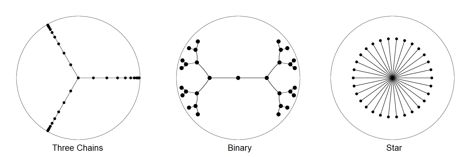
We can see where hyperbolic embeddings shine (short, bushy trees) and struggle (trees with long paths). Below we have three types of tree embeddings (designed to get a distortion under 0.1) with 31 nodes: the three chains tree requires twice as many bits to represent vertices. The example tree only has 31 nodes—the effect gets much worse with large graphs.
| Tree | Vertices | Max. Degree | Longest Path | Distortion | Bits of Precision |
| Three Chains | 31 | 3 | 10 | 0.01 | 50 |
| Binary | 31 | 3 | 4 | 0.01 | 23 |
| Star | 31 | 30 | 1 | 0.04 | 18 |
A few other comments about the two-step strategy for embedding graphs:
- The combinatorial construction embeds trees with arbitrarily low distortion and is very fast!
- There is a large literature on embedding general graphs into trees, so that we can apply the strategy to general graphs and inherit a large number of beautiful results including bounds on the distortion.
- We describe in the paper the explicit link between precision and dimension. It turns out that in higher dimensions, one can use fewer bits of precision to represent the numbers. How to use the higher dimensions appropriately is challenging, and we propose some techniques inspired by coding theory (a natural connection, since coding theory is all about fighting noise by separating codewords in space).
- This simple strategy is already quite useful, and it’s able to quickly generate embeddings that have higher accuracy than other approaches to hyperbolic embeddings. We can also use it to warm start our PyTorch implementation (below).
- A simple modification enables us to embed forests: select a large distance \(s\), much larger than all intra-component distances. Generate a new connected graph \(G'\) where the distances between a pair of nodes in each pair of components is set to \(s\), and embed \(G'\).
Getting It Exactly Right: From Distances to Points with Hyperbolic Multidimensional Scaling
A closely related problem is to recover a set of hyperbolic points \(x_1, x_2, \ldots, x_N\) without directly observing them. Instead, we are only shown the distances between points \(d_H(x_i,x_j)\). Our work shows we can (and how to) find these points! Even better, our technique doesn't necessarily require iteratively solving an optimization problem.
- A key technical step in the algorithm is normalizing the matrix of distances so that the center of mass of the points is at the origin. This mirrors the Euclidean solution to the problem, (multidimensional scaling, or MDS).
- Our case is more complex! In our paper we show how to center the points using a tricky but cute application of the Perron-Frobenius theorem. We call our approach hyperbolic MDS, or h-MDS.
- We study the properties of h-MDS under various noisy conditions (more technically involved!).
- We consider h-MDS’s sensitivity to noise through a perturbation analysis. Not surprisingly, h-MDS solutions that involve points near the edge of the disk are more sensitive to noise than traditional Euclidean MDS.
- We study dimensionality reduction with principal geodesic analysis (PGA), which mirrors the case in which there is stochastic noise around the hyperplane.
PyTorch FTW
We used the insights from our study to build a scalable PyTorch-based implementation for generating hyperbolic embeddings. Our implementation minimizes a loss function based on the hyperbolic distance; a key idea is to use the squared hyperbolic distance for the loss function, as the derivative of the hyperbolic distance function contains a singularity.
Even better—our approaches (combinatorial, h-MDS) can be used to warm-start the PyTorch implementation.
You can try producing your own hyperbolic embeddings with our code!
Takeaways:
- Hyperbolic space is awesome and has many cool properties,
- These properties make it possible to embed graphs very well.
- There are fast ways to embed (combinatorial), optimal solutions (h-MDS), and lots of interesting theory!
- Try our (preliminary!) code and check out our paper for all the details.
Data Release
In our website, we release our hyperbolic entity embeddings in GloVe format that can be further integrated into applications related to knowledge base completion or can be supplied as features into various NLP tasks such as Question Answering. We provide the hyperbolic embeddings for chosen hierarchies from WordNet, Wikidata and MusicBrainz and also evaluate the intrinsic quality of the embeddings through hyperbolic-analogues of "similarity" and "analogy".
We thank Charles Srisuwananukorn and Theo Rekatsinas for their helpful suggestions.