Accelerated Stochastic Power Iteration

by Christopher De Sa, Bryan He, Ioannis Mitliagkas, Christopher Ré, and Peng Xu
and referencing work by many other members of Hazy Research 29 Aug 2017

Surprisingly, standard acceleration doesn’t always work for stochastic PCA. We provide a very simple stochastic PCA algorithm, based on adding a momentum term to the power iteration, that achieves the optimal sample complexity and an accelerated iteration complexity in terms of the eigengap. Importantly, it is embarrassingly parallel, allowing accelerated convergence in terms of wall-clock time. Our results hinge on a tight variance analysis of a stochastic two-term matrix recurrence, which implies acceleration for a wider class of non-convex problems.

Principal component analysis (PCA) is one of the most powerful tools in machine learning. It is used in practically all data processing pipelines to allow data to be compressed and visualized. When Gene Golub and William Kahan presented a practical SVD algorithm for in 1964 they were set for life.

The current simplicity vs speed trade-off

Currently, no simple methods achieve an accelerated convergence rate in the stochastic setting.

Classic methods, like the extremely simple power iteration and the Lanczos algorithm, achieve linear rates with respect to the target accuracy, ε. Lanczos is fast, achieving an accelerated rate: the number of iterations (full passes over the data) only depends on the square root of the eigengap, Δ, between the top two eigenvalues. However, doing full passes over the data is not practical for large-scale applications. State-of-the-art stochastic PCA algorithms only iterate on a handful of samples at a time, which is much more practical and makes large-scale PCA possible. This is extremely simple and effective, resulting in popular industry use.

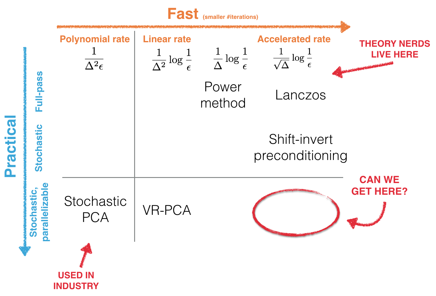
Iteration complexity—the number of embarassingly parallel steps required to reach the solution—tells us how fast an algorithm is when run on a massively parallel system. None of the simple methods for stochastic PCA achieve the accelerated rate of full-pass Lanczos. Recently, work based on shift-invert preconditioning achieved this accelerated rate; however, this method is complex and difficult to run in parallel.

QUESTION: Do we really need these complex methods to get acceleration? Let's just apply some good old momentum and go home. The optimization zeitgeist says we can accelerate anything!!

Our results

Turns out it's not that simple, but it is possible! We wrote a paper about it. In this post, we summarize the following results:

Applying acceleration techniques from optimization to the (full-pass) power method achieves quadratic acceleration. Specifically, we get this improvement by adding a momentum term.
Naively adding momentum in the stochastic setting does not always yield acceleration!
However, we can design stochastic versions of the full-pass accelerated method that are guaranteed to be accelerated. Our novel variance analysis, based on orthogonal polynomials, proves that we can achieve acceleration for small, but non-zero, variance in the iterates.
We describe two algorithms that ensure this condition holds. The first one uses a mini-batch approach, and the second one uses SVRG-style variance reduction. In the latter case the batch-size is independent of the target accuracy, ε. This means that simple methods are enough to get the optimal sample complexity and an accelerated iteration complexity.

Unlike previous methods, each iteration of our algorithms is parallelizable. Deployed in parallel, our methods achieve true acceleration in wall clock time!

The notebooks reproducing our experiments can be found here.

These theoretical insights are part of a broader body of work. In YellowFin, we use this theoretical understanding of momentum to provide an automatic tuner for SGD that is competitive with state-of-the-art adaptive methods on training ResNets and LSTMs.

Accelerating the Power Method

The goal of PCA is to find the top eigenvector of a symmetric positive semidefinite matrix $A\in \mathbb R^{d\times d}$, often known as the sample covariance matrix. A popular way to find this is the power method, which iteratively runs the update $\mathbf{w}_{t+1} = A \mathbf{w}_t$ and converges to the top eigenvector in $\tilde{\mathcal O}(1/\Delta)$ steps, where $\Delta$ is the eigen-gap between the top two eigenvalues of $A$. As we mentioned earlier, this convergence is really slow if the matrix is poorly conditioned.

Adding momentum to the power method achieves quadratic acceleration.

Motivated by momentum methods used to accelerate convex optimization, we tried to apply momentum to the power method. In particular, we tried replacing the power method update with $$\mathbf{w}_{t+1} = A\mathbf{w}_t - \beta \mathbf{w}_{t-1},$$ where the extra $\beta \mathbf{w}_{t-1}$ is the analogue of the momentum term from convex optimization. Given its similarity to known acceleration schemes, perhaps it is not surprising that with appropriate settings of $\beta$, the momentum update converges in $\tilde{\mathcal O}(1/\sqrt\Delta)$ steps.

The magic behind the scenes is the Chebyshev polynomials. The entire dynamics of the momentum update can be captured by the two-term recurrence of the (scaled) Chebyshev polynomials $$p_{t+1}(x) = x p_t(x) - \beta p_{t-1}(x).$$ In particular, the Chebyshev polynomial evaluated at $\lambda_i$ gives the decay of the eigen-direction corresponding to eigenvalue $\lambda_i$. To help illustrate the effect of momentum on eigenvectors with different eigenvalues, we show the (scaled) Chebyshev polynomials at $t=100$ for several different momentum parameters. This lets us visually compare how quickly different eigenvectors will decay.

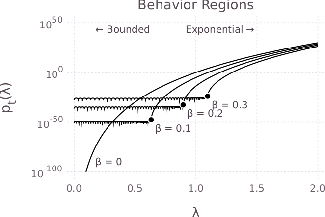
From this, we can see that the (scaled) Chebyshev polynomials have two regions: a bounded region and an exponential region. In the bounded region, the Chebyshev polynomials are small, and in the exponential region, the Chebyshev polynomial grows rapidly.

For power iteration, where $\beta = 0$, the corresponding polynomial is $p_t(\lambda) = \lambda^t$. The recurrence reduces mass on small eigenvalues quickly. However, eigenvalues near the largest eigenvalue decay relatively slowly, yielding slow convergence.

As $\beta$ is increased, an elbow appears in $p_t(\lambda)$. For values of $\lambda$ smaller than the knee, $p_t(\lambda)$ remains small, which implies that these eigenvalues decay quickly. For values of $\lambda$ greater than the knee, $p_t(\lambda)$ grows rapidly, which means that these eigenvalues will remain. By selecting a $\beta$ value that puts the elbow close to $\lambda_2$ so that $\lambda_1$ can stay as far as possible away from the calm region, our recurrence quickly eliminates mass on all but the largest eigenvector.

Generalizing to the Stochastic Setting

As we mentioned before, we would like our method to work for the stochastic setting, which is the streaming PCA setting. Given the simplicity of the deterministic method we just discussed, one natural option is to add momentum to the stochastic power method (also known as Oja’s algorithm), rather than the deterministic power method, leading to the recurrence $\mathbf{w}_{t+1} = (I + \eta\tilde A_t) \mathbf{w}_t - \beta \mathbf{w}_{t-1}.$ To test this approach, we run this update on a randomly generated matrix.

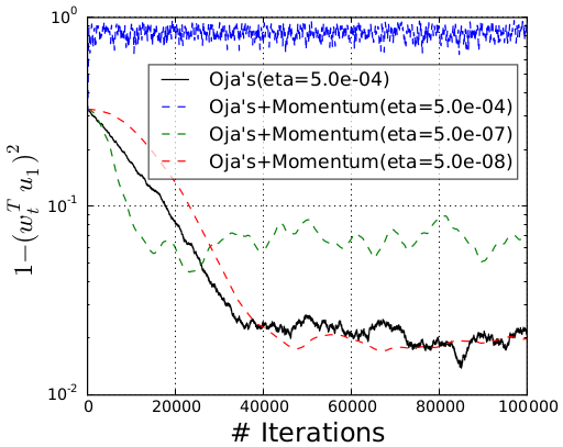
However, this is what we get from the experiment: even after searching for a good learning rate $\eta$, we did NOT obtain acceleration by adding momentum!

Naively adding momentum in the stochastic setting does not always work!

What's wrong? From the experiment, we see that adding momentum does accelerate convergence to the noise ball (For a constant step size scheme, the stochastic algorithm won't converge to the true solution. Instead, it converges to a level where it fluctuates, and we refer to the fluctuation level as the noise ball). However, it also increases the size of the noise ball. We have to decrease the step size to remedy this increase in the noise ball, but this roughly cancels out the acceleration from momentum. This phenomenon has independently been observed for stochastic optimization. Now, we need to figure out what exactly is happening in the stochastic case, since we know we can obtain quadratic acceleration in the deterministic case.

A simple statistic to quantify the stochasticity of the problem is the variance of the iterates. Can we characterize the connection between the variance and momentum parameter? Yes we can! And once again, the magic bullet is the Chebyshev polynomials, which has a closed-form expression to help with the variance analysis. Specifically, the stochastic update can be reduced to analyzing the stochastic matrix sequence $$F_{t+1} = A_{t+1} F_t - \beta F_{t-1},$$ where $A_{t}$ is an i.i.d random matrix with $\mathbb{E}[A_t] = A$.

You have to have low variance for momentum to work in the stochastic setting.

It turns out that we can obtain an almost exact expression for the variance of each iterate $F_t$, which we show in our work. There are two technical tricks that help the analysis:

The first trick is to use the Kronecker product to characterize the covariance of the random matrix. Since this is a linear recurrence, the second order (and in fact, any order) moment also follows a linear recurrence.

The second trick is to exploit the known closed-form expression of Chebyshev polynomials.

With these two points, we can build up the variance bound, which can then be used for any further analysis for momentum methods in the stochastic setting. Using this, we are able to show that under the condition of low variance, this momentum scheme is able to achieve acceleration.

How to Control the Variance

The variance condition for obtaining acceleration with momentum over the stochastic power method is pretty strict. However, there are several ways that the variance of the iterates can be controlled to obtain acceleration more generally.

You can get acceleration in the stochastic setting by controlling the variance.

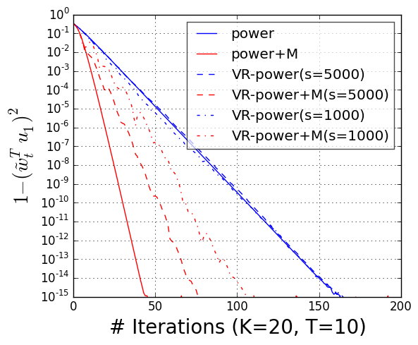
We consider two common ways to lower the variance: mini-batching and variance reduction. Mini-batching is a popular way to speed up computation in stochastic optimization and is embarrassingly parallelizable. By using large enough mini-batch sizes, we can guarantee acceleration from momentum. However, to achieve very accurate solutions, the required mini-batch size grows in size.

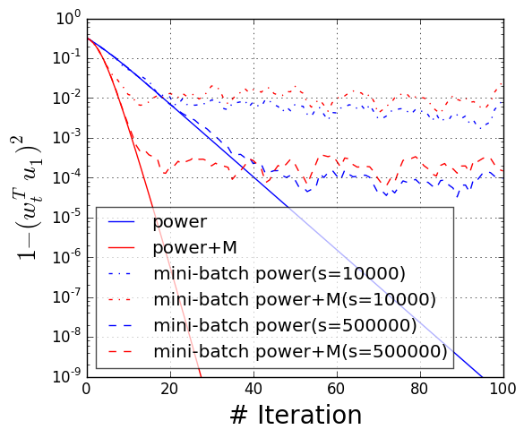
The second technique we consider is variance reduction, as in SVRG. Variance reduction makes it possible to use a batch size that does not grow when we increase accuracy. By using a small number of full passes (possible when the data is not sampled at random but available in a fixed dataset), variance reduction significantly reduces the required mini-batch size while still achieving an accelerated linear convergence.

Next Steps

Our variance analysis generalizes as a tool for other problems. In particular, these techniques should work for problems such as randomized iterative solvers for linear systems and convex quadratic optimization problems.

Our work points out two interesting directions:

Can we extend our convergence analysis to the stochastic convex optimization setting? For general convex objectives, the difficulty comes from the fact that the gradient is no longer a linear or affine function of the iteration. Can we characterize the behavior of momentum with respect to the noise of the system like in the streaming PCA setting?
PCA is intrinsically a non-convex optimization problem, so can we extend the momentum scheme further to other non-convex problems where we can obtain acceleration under certain conditions?